
Static and Dynamic Characteristics of Instruments – Complete Guide for Instrument Technicians
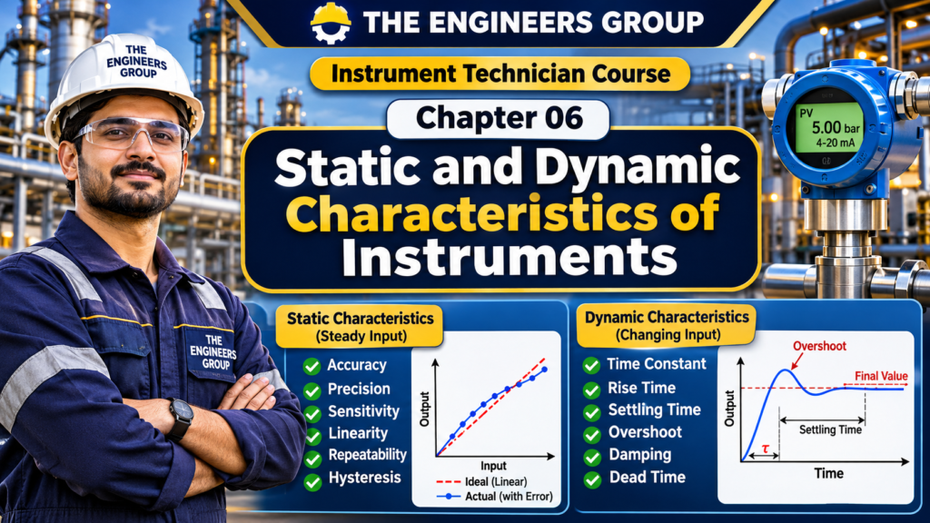
Chapter 06 – Free Instrument Technician Course
Table of Contents
- Introduction to Instrument Characteristics
- What Are Static Characteristics?
- Accuracy
- Precision
- Sensitivity
- Linearity
- Repeatability
- Reproducibility
- Resolution
- Hysteresis
- Dead Zone and Threshold
- Drift and Stability
- What Are Dynamic Characteristics?
- Speed of Response
- Time Constant
- Rise Time and Settling Time
- Overshoot and Damping
- Dead Time
- First-Order and Second-Order Instrument Response
- Static vs Dynamic Characteristics
- Practical Industrial Examples
- Importance of Instrument Characteristics
- Common Problems and Troubleshooting
- Instrument Technician Interview Questions and Answers
- Multiple Choice Questions (MCQs)
- Chapter Summary
- What Is Next?
1. Introduction to Instrument Characteristics
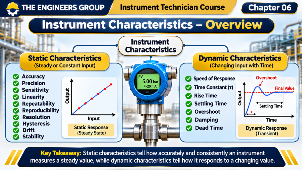
Static and dynamic characteristics of instruments are important factors in evaluating the performance of industrial measuring instruments. They help Instrument Technicians and Maintenance Engineers understand how accurately, consistently and quickly an instrument responds to different process conditions.
Every measuring instrument has certain performance characteristics that determine how well it measures a physical quantity such as pressure, temperature, flow, level or speed.
For example, consider a pressure transmitter installed on an industrial pipeline. It must:
- Measure pressure accurately.
- Produce consistent readings under the same conditions.
- Respond properly when pipeline pressure changes.
- Maintain stable output over time.
- Detect small changes in the measured pressure.
These performance properties are known as the characteristics of instruments.
Instrument characteristics are broadly classified into two categories:
- Static Characteristics
- Dynamic Characteristics
Understanding both categories helps Instrument Technicians, Maintenance Engineers and Calibration Engineers evaluate instrument performance and identify measurement problems.
2. What Are Static Characteristics?
Static characteristics describe the performance of an instrument when the measured quantity is constant or changes very slowly with time.
In simple words, static characteristics explain how accurately and consistently an instrument measures a steady input.
For example:
A pressure transmitter has a measuring range of 0–10 bar. If the actual pressure remains constant at 5 bar, the transmitter should provide a stable and correct output corresponding to that pressure.
The following are important static characteristics:
- Accuracy
- Precision
- Sensitivity
- Linearity
- Repeatability
- Reproducibility
- Resolution
- Hysteresis
- Dead Zone
- Threshold
- Drift
- Stability
Let’s understand each characteristic with industrial examples.
3. Accuracy
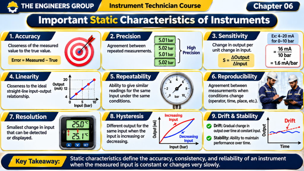
Accuracy is the closeness of an instrument’s measured value to the true or reference value.
In simple words, accuracy tells us how close the instrument reading is to the actual measurement.
Practical Example:
Suppose a calibrated pressure reference shows 5.00 bar.
A pressure transmitter indicates 4.98 bar.
The measurement error is:
Error = Measured Value − Reference Value
Error = 4.98 − 5.00
Error = −0.02 bar
The negative sign indicates that the instrument is reading below the reference value.
A smaller measurement error generally indicates better accuracy.
Important: Accuracy specifications may be expressed as a percentage of full scale, reading or span. Always check the manufacturer’s datasheet to understand the stated accuracy specification.
4. Precision
Precision describes how closely repeated measurements agree with each other under the same measurement conditions.
In simple words, precision tells us whether an instrument gives nearly the same reading when the same measurement is repeated.
Practical Example:
Suppose a pressure reference is maintained at 5 bar and a transmitter gives the following readings:
- Reading 1: 5.01 bar
- Reading 2: 5.02 bar
- Reading 3: 5.01 bar
- Reading 4: 5.02 bar
These readings are close to each other, indicating good repeatability and precision.
However, precision does not automatically mean accuracy. An instrument may repeatedly show almost the same incorrect value.
Remember:
- Accuracy = Closeness to the reference value.
- Precision = Closeness among repeated readings.
5. Sensitivity
Sensitivity is the ratio of the change in instrument output to the corresponding change in input.
It indicates how much the output changes when the measured quantity changes.
Formula:
Sensitivity = Change in Output / Change in Input
Practical Example:
A pressure transmitter measures 0–10 bar and produces a 4–20 mA output.
Input change = 10 bar
Output change = 20 − 4 = 16 mA
Sensitivity = 16 / 10
Sensitivity = 1.6 mA/bar
This means the output changes by 1.6 mA for every 1 bar increase in pressure within the specified linear range.
Sensitivity is important when selecting instruments for applications that require the detection of small measurement changes.
6. Linearity
Linearity describes how closely an instrument’s actual input-output relationship follows its specified ideal straight-line relationship.
In a linear instrument, equal changes in input produce proportional changes in output.
Practical Example:
Consider a pressure transmitter with a range of 0–10 bar and an output of 4–20 mA.
| Pressure | Expected Output |
|---|---|
| 0 bar | 4 mA |
| 2.5 bar | 8 mA |
| 5 bar | 12 mA |
| 7.5 bar | 16 mA |
| 10 bar | 20 mA |
If the transmitter follows the specified straight-line relationship, it demonstrates linear behavior.
In practical instruments, small deviations from the ideal line may occur. The manufacturer normally specifies the permitted non-linearity.
💬 NEED GUIDANCE ?
Contact THE ENGINEERS GROUP for eBook details, course information and learning support.
MESSAGE US ON WHATSAPP7. Repeatability
Repeatability is the ability of an instrument to produce similar readings when the same input is applied repeatedly under the same operating conditions.
These conditions generally include:
- Same instrument
- Same operator
- Same measurement method
- Same environmental conditions
- Short time interval
Practical Example:
A temperature transmitter is tested at a constant reference temperature of 100°C.
Repeated readings are:
- 100.1°C
- 100.1°C
- 100.2°C
- 100.1°C
The close agreement indicates good repeatability.
Repeatability is important in calibration, quality control and process monitoring.
8. Reproducibility
Reproducibility describes the agreement between measurement results when measurement conditions change in specified ways.
These changes may include:
- Different operators
- Different measurement equipment
- Different laboratories
- Different locations
- Different measurement times
Practical Example:
Two technicians independently test the same pressure instrument using suitable calibrated reference equipment.
Technician A obtains 5.01 bar.
Technician B obtains 5.02 bar.
The close agreement indicates good reproducibility under the tested conditions.
Difference:
- Repeatability: Same conditions.
- Reproducibility: Changed measurement conditions.
9. Resolution
Resolution is the smallest change in the measured quantity that an instrument can detect or display.
In simple words, resolution tells us how small a change the instrument can show.
Practical Example:
A digital temperature indicator displays readings with a resolution of 0.1°C.
It may display:
- 25.0°C
- 25.1°C
- 25.2°C
It cannot display a smaller increment than 0.1°C through that display resolution.
Important: Resolution and accuracy are different. An instrument may display many decimal places but still have significant measurement error.
10. Hysteresis
Hysteresis occurs when an instrument gives different outputs for the same input depending on whether the input is increasing or decreasing.
In simple words, the output depends partly on the direction from which the measurement point is approached.
Practical Example:
A pressure transmitter is tested at 5 bar.
During increasing pressure, the output is 12.1 mA.
During decreasing pressure, the output is 11.9 mA.
The difference is:
Hysteresis Difference = 12.1 − 11.9
Hysteresis Difference = 0.2 mA
This difference indicates hysteresis at the tested pressure point.
Possible causes include:
- Mechanical friction
- Backlash
- Material deformation
- Mechanical wear
- Sensor-related effects
Hysteresis is commonly checked during instrument calibration by testing the instrument in both increasing and decreasing directions.
11. Dead Zone and Threshold
Dead Zone
Dead zone is a range of input changes over which the instrument output does not respond noticeably.
Example:
A control valve positioner receives a small change in control signal, but the valve stem does not move because of friction or mechanical resistance.
This behavior may indicate a dead zone or related mechanical problem.
Threshold
Threshold is the minimum input required to produce a detectable output response from an instrument.
Example:
A sensor may not produce a detectable output change until the measured pressure increases beyond a particular minimum value.
Threshold is important when selecting instruments for low-pressure or small-signal applications.
12. Drift and Stability
Drift
Drift is the gradual change in an instrument’s output over time when the actual input remains constant.
Common causes include:
- Temperature variations
- Ageing of electronic components
- Sensor degradation
- Mechanical wear
- Changes in power supply
- Environmental conditions
Practical Example:
A pressure transmitter is exposed to a constant reference pressure of 5 bar.
Initially, it indicates 5.00 bar.
After several months, it indicates 5.08 bar under the same reference conditions.
This may indicate measurement drift and the instrument should be investigated and checked against a suitable reference.
Stability
Stability is the ability of an instrument to maintain its performance characteristics over time under specified operating conditions.
An instrument with good stability maintains consistent measurement performance over its service period.
Difference:
- Drift describes an unwanted change in output over time.
- Stability describes the ability to maintain consistent performance.
13. What Are Dynamic Characteristics?
Dynamic characteristics describe how an instrument responds when the measured quantity changes with time.
In industrial processes, pressure, temperature, flow and level are not always constant. They may increase, decrease or fluctuate continuously.
A measuring instrument should respond to these changes within an acceptable time and with suitable accuracy.
Practical Example:
Consider a temperature sensor installed in an industrial furnace.
When the furnace temperature increases from 100°C to 200°C, the sensor does not necessarily indicate 200°C immediately.
It takes some time to respond to the temperature change.
The way the sensor responds during this period is described by its dynamic characteristics.
Important dynamic characteristics include:
- Speed of Response
- Time Constant
- Rise Time
- Settling Time
- Overshoot
- Damping
- Dead Time
- Dynamic Error
14. Speed of Response
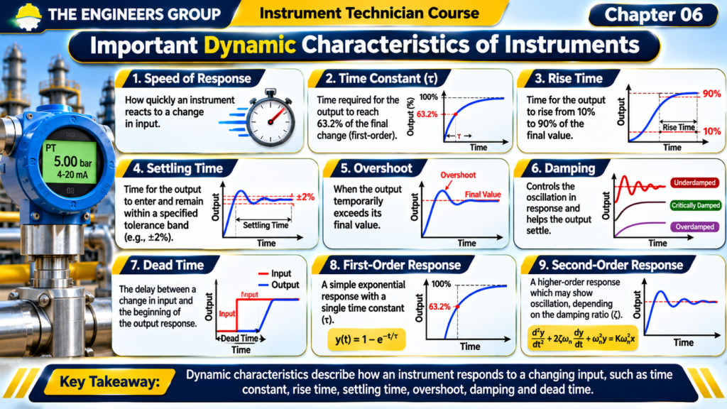
Speed of response describes how quickly an instrument reacts when its input changes.
A faster instrument responds more quickly to changes in the measured variable.
Practical Example:
Consider two temperature sensors installed in similar process conditions.
Sensor A responds to a temperature change in 5 seconds.
Sensor B responds to the same change in 20 seconds.
Sensor A has a faster response under the tested conditions.
Fast response is important in applications where process variables change rapidly, such as:
- Gas pressure monitoring
- Fast-flowing process lines
- Turbine monitoring
- Rapid temperature changes
- Dynamic control systems
However, the required response time depends on the process. An extremely fast response is not always necessary.
15. Time Constant
Time constant is an important dynamic characteristic, especially for first-order measuring instruments.
For a first-order instrument subjected to a step change in input, the time constant is the time required for the output to reach approximately 63.2% of its total final change.
Formula:
For a first-order response:
Output Response = 1 − e^(-t/τ)
Where:
- t = Elapsed time
- τ = Time constant
- e = Exponential constant
Practical Example:
A temperature sensor experiences a sudden temperature change from 0°C to 100°C.
If its time constant is 10 seconds, the output reaches approximately 63.2% of the total change after 10 seconds.
Therefore:
Output after 10 seconds = 63.2°C
This assumes an ideal first-order response and a zero initial reading.
Important:
- Smaller time constant = Faster first-order response.
- Larger time constant = Slower first-order response.
16. Rise Time and Settling Time
Rise Time
Rise time is the time taken by an instrument’s output to rise from a specified lower percentage to a specified higher percentage of its final value.
A common definition for control-system step response is the time taken to rise from 10% to 90% of the final value.
The exact definition should always be checked because different specifications may use different limits.
Settling Time
Settling time is the time required for an instrument’s output to enter and remain within a specified tolerance band around its final value.
For example, an instrument may be considered settled when its output remains within ±2% of its final value.
Practical Example:
A pressure measurement system receives a sudden pressure change.
Its output initially changes, then gradually stabilizes around the final value.
The time required to remain within the specified tolerance band is its settling time.
17. Overshoot and Damping
Overshoot
Overshoot occurs when an instrument or measurement system temporarily exceeds its final steady-state value after an input change.
Practical Example:
A measurement system is expected to settle at 100 units.
Its output temporarily rises to 110 units before returning to 100 units.
Overshoot = 110 − 100
Overshoot = 10 units
Percentage Overshoot:
% Overshoot = (Peak Value − Final Value) / Final Value × 100
% Overshoot = (110 − 100) / 100 × 100
% Overshoot = 10%
Damping
Damping describes how oscillations in a system decrease over time.
It affects how quickly the system settles after a disturbance or input change.
Common response behaviors include:
- Underdamped: The output oscillates before settling.
- Critically Damped: The system reaches its final value quickly without oscillation in the ideal second-order case.
- Overdamped: The system approaches its final value slowly without oscillation.
Damping is particularly important in mechanical measuring systems and control systems.
18. Dead Time
Dead time is the delay between a change in input and the beginning of the instrument’s output response.
Practical Example:
A process pressure changes at a pipeline location, but the measurement system begins showing the change after a short delay because of the measurement arrangement or signal transmission path.
The delay before the response begins is known as dead time.
Possible sources include:
- Long impulse lines
- Sample transport delays
- Signal processing delays
- Communication delays
- Sensor and measurement arrangement
Dead time is important in process control because excessive delay can affect control-loop performance.
19. First-Order and Second-Order Instrument Response
Dynamic measuring systems are often described using mathematical models.
First-Order System
A first-order system can be represented by:
τ(dy/dt) + y = Kx
Where:
- τ = Time constant
- y = Output
- x = Input
- K = Steady-state gain
- dy/dt = Rate of change of output
A first-order system generally approaches its final value exponentially after a step input.
Examples may include certain temperature sensors and thermal measurement arrangements under suitable operating conditions.
Second-Order System
A second-order system can be represented by:
(d²y/dt²) + 2ζωₙ(dy/dt) + ωₙ²y = Kωₙ²x
Where:
- ζ = Damping ratio
- ωₙ = Natural angular frequency
- x = Input
- y = Output
- K = Steady-state gain
Second-order systems may show oscillatory behavior depending on their damping ratio.
Examples include certain mechanical measuring systems, vibration sensors and moving-element instruments.
The actual dynamic behavior depends on the instrument design and operating conditions.
MASTER INDUSTRIAL
INSTRUMENTATION
Build your technical knowledge with our Instrument Technician E-book – English Edition.
Instrument Technician E-book (English Edition)
Learn essential industrial instrumentation concepts, measurement systems, calibration and troubleshooting in one practical guide.
WHAT YOU WILL LEARN:
- Fundamentals of Industrial Instrumentation
- Pressure, Temperature, Flow and Level Measurement
- Sensors, Transmitters and Control Valves
- Instrument Calibration and Troubleshooting
- PLC, SCADA and Industrial Control Systems
- Essential Instrumentation Interview Preparation
SPECIAL OFFER PRICE
Digital eBook – English Edition
Secure online payment • Digital delivery via email
No physical book will be delivered.
Ideal For:
ITI & Diploma Students | B.Tech Graduates | Instrument Technicians | Junior Engineers
Learn • Practice • Improve Your Engineering Skills
THE ENGINEERS GROUP
20. Static vs Dynamic Characteristics
| Static Characteristics | Dynamic Characteristics |
|---|---|
| Describe performance with constant or slowly changing input | Describe performance with time-varying input |
| Focus on steady-state measurement behavior | Focus on response to changing input |
| Accuracy | Speed of response |
| Precision | Time constant |
| Sensitivity | Rise time |
| Linearity | Settling time |
| Repeatability | Overshoot |
| Reproducibility | Damping |
| Resolution | Dead time |
| Hysteresis | Dynamic response |
Understanding static and dynamic characteristics of instruments is essential for selecting, testing, calibrating and maintaining industrial measurement systems. These characteristics help engineers evaluate measurement accuracy, repeatability, response time and overall instrument performance.
Remember:
Static characteristics tell us how well an instrument measures a steady value.
Dynamic characteristics tell us how well an instrument responds to a changing value.
21. Practical Industrial Examples
Example 1: Pressure Transmitter
A pressure transmitter installed on a process pipeline should:
- Measure pressure accurately.
- Provide repeatable readings.
- Maintain linear output.
- Respond to pressure changes within the required time.
- Maintain stable performance over time.
Static characteristics help evaluate its steady-state measurement performance.
Dynamic characteristics help evaluate its response to changing pipeline pressure.
Example 2: RTD Temperature Sensor
An RTD installed in a process tank measures the process temperature.
Important static characteristics include:
- Accuracy
- Repeatability
- Resolution
- Stability
Important dynamic characteristics include:
- Response time
- Time constant
- Settling time
The RTD installation method, thermowell and process conditions can influence the overall response time.
Example 3: Flow Transmitter
A flow transmitter measures liquid or gas flow in a pipeline.
Static performance is important when flow remains stable.
Dynamic performance is important when flow changes rapidly due to pump speed changes, valve operation or process demand.
Example 4: Level Transmitter
A level transmitter monitors liquid level in a storage tank.
Static characteristics help determine the quality of steady level measurement.
Dynamic characteristics help evaluate how the measurement responds when the tank is filling or emptying.
22. Importance of Instrument Characteristics
Understanding instrument characteristics is important for several reasons:
- Instrument Selection: Helps select the correct instrument for a particular process.
- Measurement Reliability: Helps evaluate whether readings are consistent and dependable.
- Calibration: Helps identify errors and verify instrument performance.
- Troubleshooting: Helps identify drift, hysteresis, poor repeatability and slow response.
- Process Control: Helps ensure measurement systems respond appropriately to process changes.
- Plant Safety: Supports reliable monitoring of critical process variables.
- Maintenance Planning: Helps identify performance degradation and the need for inspection or calibration.
23. Common Problems and Troubleshooting
| Problem | Possible Cause | Recommended Check |
|---|---|---|
| Incorrect reading | Calibration error or sensor fault | Compare with a calibrated reference |
| Unstable reading | Electrical noise or loose connection | Check wiring, shielding and grounding |
| Slow response | Sensor lag or process connection issue | Check sensor installation and response specification |
| Different readings in increasing and decreasing direction | Hysteresis or mechanical friction | Perform an increasing and decreasing calibration test |
| Gradual output change | Drift or sensor ageing | Compare with a reference and review calibration history |
| Small changes not detected | Limited resolution or threshold | Check instrument resolution and range |
| Output oscillation | Process fluctuation or dynamic response issue | Check process behavior and measurement-system response |
Always follow the instrument manufacturer’s instructions and plant safety procedures before inspection or maintenance.
24. Instrument Technician Interview Questions and Answers
Q1. What are the characteristics of measuring instruments?
Answer: They are performance properties that describe how an instrument measures a physical quantity. They are broadly classified into static and dynamic characteristics.
Q2. What are static characteristics?
Answer: Static characteristics describe instrument performance when the measured input is constant or changes very slowly with time.
Q3. What are dynamic characteristics?
Answer: Dynamic characteristics describe how an instrument responds when the measured input changes with time.
Q4. What is accuracy?
Answer: Accuracy is the closeness of a measured value to the true or reference value.
Q5. What is precision?
Answer: Precision describes the closeness of agreement between repeated measurements under specified conditions.
Q6. What is sensitivity?
Answer: Sensitivity is the ratio of change in output to the corresponding change in input.
Q7. What is linearity?
Answer: Linearity describes how closely an instrument’s actual input-output relationship follows its specified ideal straight-line relationship.
Q8. What is repeatability?
Answer: Repeatability is the ability of an instrument to produce similar readings when the same input is applied repeatedly under the same conditions.
Q9. What is reproducibility?
Answer: Reproducibility describes the agreement between measurements when specified measurement conditions change.
Q10. What is hysteresis?
Answer: Hysteresis occurs when an instrument produces different outputs for the same input depending on whether the input is increasing or decreasing.
Q11. What is resolution?
Answer: Resolution is the smallest change in input that can be detected or displayed by an instrument.
Q12. What is drift?
Answer: Drift is the gradual change in instrument output over time when the actual input remains constant.
Q13. What is time constant?
Answer: For a first-order instrument, time constant is the time required for its output to reach approximately 63.2% of the total final change after a step input.
Q14. What is overshoot?
Answer: Overshoot occurs when the output temporarily exceeds its final steady-state value after an input change.
Q15. What is the difference between static and dynamic characteristics?
Answer: Static characteristics describe performance under constant or slowly changing inputs, whereas dynamic characteristics describe performance when the input changes with time.
⚙️ 100 INSTRUMENTATION INTERVIEW Q&A
Prepare for your Instrument Technician and Instrumentation Engineer interviews with 100 important technical questions and answers.
📥 DOWNLOAD 100 INTERVIEW Q&A PDFFREE STUDY MATERIAL | THE ENGINEERS GROUP
25. Multiple Choice Questions (MCQs)
Q1. Instrument characteristics are broadly classified into which two categories?
A. Electrical and Mechanical
B. Static and Dynamic
C. Analog and Digital
D. Pressure and Temperature
Correct Answer: B. Static and Dynamic
Q2. Which characteristic describes the closeness of a measured value to the true value?
A. Precision
B. Sensitivity
C. Accuracy
D. Resolution
Correct Answer: C. Accuracy
Q3. Which characteristic describes agreement between repeated readings under the same conditions?
A. Repeatability
B. Drift
C. Hysteresis
D. Threshold
Correct Answer: A. Repeatability
Q4. Sensitivity is calculated as:
A. Input / Output
B. Change in Output / Change in Input
C. Output × Input
D. Error / Range
Correct Answer: B. Change in Output / Change in Input
Q5. Which characteristic describes how closely an instrument follows its ideal straight-line relationship?
A. Stability
B. Linearity
C. Drift
D. Precision
Correct Answer: B. Linearity
Q6. Different outputs for the same input during increasing and decreasing measurement indicate:
A. Resolution
B. Accuracy
C. Hysteresis
D. Sensitivity
Correct Answer: C. Hysteresis
Q7. The smallest detectable change in measurement is known as:
A. Range
B. Resolution
C. Drift
D. Stability
Correct Answer: B. Resolution
Q8. Gradual change in output over time at constant input is called:
A. Drift
B. Linearity
C. Precision
D. Threshold
Correct Answer: A. Drift
Q9. Which characteristic describes the response of an instrument to changing input?
A. Accuracy
B. Static characteristic
C. Dynamic characteristic
D. Resolution
Correct Answer: C. Dynamic characteristic
Q10. For an ideal first-order instrument, the output reaches approximately what percentage of its final change after one time constant?
A. 25%
B. 50%
C. 63.2%
D. 100%
Correct Answer: C. 63.2%
Q11. Which term describes the time required for the output to enter and remain within a specified tolerance band?
A. Rise time
B. Settling time
C. Dead time
D. Drift
Correct Answer: B. Settling time
Q12. When output temporarily exceeds its final value, the condition is called:
A. Damping
B. Dead zone
C. Overshoot
D. Resolution
Correct Answer: C. Overshoot
Q13. Which term describes the delay before an instrument begins responding to an input change?
A. Dead time
B. Sensitivity
C. Accuracy
D. Repeatability
Correct Answer: A. Dead time
Q14. Which system may show oscillatory behavior depending on its damping ratio?
A. First-order system only
B. Second-order system
C. Static system only
D. Digital display only
Correct Answer: B. Second-order system
Q15. Which characteristic is most directly related to maintaining consistent measurement performance over time?
A. Stability
B. Overshoot
C. Dead time
D. Rise time
Correct Answer: A. Stability
26. Chapter Summary
In this chapter, we studied the static and dynamic characteristics of industrial measuring instruments.
Important points to remember:
- Static characteristics describe performance under constant or slowly changing input.
- Dynamic characteristics describe performance under changing input.
- Accuracy indicates closeness to a reference value.
- Precision describes agreement among repeated measurements.
- Sensitivity is the ratio of output change to input change.
- Linearity describes how closely the instrument follows its ideal input-output relationship.
- Repeatability and reproducibility describe measurement agreement under specified conditions.
- Resolution is the smallest detectable measurement change.
- Hysteresis depends on the direction of input change.
- Drift is a gradual output change over time.
- Time constant describes the response of a first-order instrument.
- Rise time, settling time, overshoot and damping describe important aspects of dynamic response.
A good Instrument Technician should understand these characteristics to evaluate instrument performance, perform calibration checks and troubleshoot industrial measurement systems.
27. What Is Next?
Chapter 07 – Sensors, Transducers and Transmitters
In the next chapter, we will learn:
- What is a Sensor?
- What is a Transducer?
- What is a Transmitter?
- Difference Between Sensor, Transducer and Transmitter
- Types of Industrial Sensors
- Working Principles and Practical Applications
- Industrial Examples and Interview Questions
Continue learning with THE ENGINEERS GROUP – Free Instrument Technician Course.
Learn • Practice • Improve Your Engineering Skills
CONNECT WITH THE ENGINEERS GROUP
Learn. Practice. Improve. Grow.
📘 EXPLORE OUR EBOOK 💬 CONTACT US ON WHATSAPP ▶️ SUBSCRIBE ON YOUTUBE FOLLOW US ON FACEBOOKTHE ENGINEERS GROUP
Free Engineering Education for Everyone